← Fourier as a bank of correlators
What we do in this lesson
There is no new physics today — the DFT formula is the same as in the previous lesson. The goal of the lesson is to make the formula less abstract and to answer the practical questions that come up when you actually calculate a spectrum in code:
- We go through the DFT formula by hand on a toy example of four numbers, step by step, with no steps skipped.
- We find out what the output index means and in which order
np.fft.fftreturns the results — this is the first thing that confuses people who work with NumPy. - We see why nobody calculates the DFT directly from the formula for long records.
- We understand the main idea of the FFT — it is not new mathematics, but a method to reuse results that are already calculated instead of calculating from zero.
Back to the correlator formula
In the previous lesson, one correlator tested one frequency: it multiplied the signal samples by the reference rotation and added the results. The DFT is simply a bank of such correlators that work at the same time, one for each frequency of the grid:
Here is the index of the input sample in time, and is the index of the output bin in frequency. Not one symbol of the formula changed — we only repeat it for each from to .
We calculate the DFT by hand on four samples
We take the smallest example in which we can still see each term. Let , and let the input signal be a usual real cosine, with exactly one period in four samples:
Note: the signal itself is only four usual numbers, not vectors on a plane. But the reference signals inside each correlator are still complex — the same as in the previous lesson.
To find for a specific , multiply each sample by the related value of the reference rotation and add the four results. Here the reference rotation makes an integer number of turns in 4 steps, so its values are the four points on the circle that we already know: . We write them for all pairs in a table — these are all the reference signals that we need:
| 0 | 1 | 2 | 3 | |
|---|---|---|---|---|
| 0 | ||||
| 1 | ||||
| 2 | ||||
| 3 |
The table row with index is the reference signal of bin . Now, for each , we multiply this row by the input element by element and add. Note: we have , so these two terms become zero on their own, and we only need to calculate the contribution from and :
- :
- :
- :
- :
We get . All four numbers are real, with no imaginary part — this is not a coincidence: the input signal was real. And is exactly what the rule from the previous lesson predicts for a cosine with amplitude : each of its two components (the clockwise and the counterclockwise rotation) gives the contribution .
How to read the bin index k as a frequency
The four numbers alone tell nothing about frequencies in hertz — the formula gives the link to . We take kS/s, as before:
| 0 | 1 | 2 | 3 | |
|---|---|---|---|---|
| , Hz |
The last number looks wrong: at kS/s, the Nyquist frequency is Hz, and Hz is above it. Here the same aliasing effect operates that we studied in Part 1: on a grid of 4 samples, a rotation of Hz is the same as a rotation of Hz. Thus np.fft.fft does not show frequencies above Nyquist — instead, it gives the second half of the bins negative frequency labels:
| 0 | 1 | 2 | 3 | |
|---|---|---|---|---|
| Frequency |
This is the order in which np.fft.fft actually returns the array: first zero, then the positive frequencies in increasing order, then the negative frequencies — also in increasing order, starting from the Nyquist frequency. The Nyquist frequency itself () has the label Hz by convention, but it could equally be Hz — it is the same rotation.
This order is not convenient for a plot — we want the frequencies to increase from left to right. This is what np.fft.fftshift() does: it changes the order of the array and calculates nothing again:
| Frequency | ||||
|---|---|---|---|---|
Now we see the same as in the previous lesson: a cosine gives two equal peaks — at and at Hz. A correlator cannot tell a positive rotation from a negative one while the signal is real, so the energy always divides equally between the mirror frequencies.
Why we need a faster algorithm
For each of the bins, the DFT formula must go through all samples — this is approximately multiplications and additions. For our example with , this is operations, a very small number. But imagine a receiver that continuously makes the spectrum of an audio stream at samples per second and updates the picture many times per second — at this scale, quickly becomes too large. For a record of length (, approximately 1 second on some SDRs), the number of operations is — more than a trillion for one single spectrum.
The FFT is a fast algorithm that calculates the same sum as the DFT, but not directly. It is not a different transform and not an approximation: the FFT returns the same numbers as the DFT formula, but it gets to them by a different path.
The idea of the FFT: we use what is already calculated
The key observation is simple: if you divide a signal of length into two halves — the even and the odd samples — then each half is itself a signal of length , and you can calculate its DFT separately. When it is calculated, both outputs of the full DFT — and its “pair” — come from the same two half-length results, with a different sign on one term. Thus, instead of going through all samples again for each of the bins, we do the work only once on each half of the data and use it two times.
We write this as a formula. We write the DFT of the even samples as and the DFT of the odd samples as (both have length ):
Then you can make the full DFT of length from them like this:
This pair of equations is called a “butterfly” — both outputs come from the same pair of numbers , , only with a plus and a minus.
We check this on our example to see that the numbers do not change. The even samples are , the odd samples are . For two numbers, we calculate the DFT with the same logic as above, but with :
- ,
- — the odd samples are zero, so their DFT is also zero
We make the full result with the butterfly formula:
- ,
- ,
Again — the same as the result of the direct calculation. But instead of multiplications, it was sufficient to calculate two DFTs of two samples each and combine them with a pair of additions.
On such a small example, you cannot see the saving, but the method scales recursively: you can divide each of the two halves of length in half again in the same way, and so on, until only pieces of one sample remain (the DFT of one number is the number itself). There are levels of division, and at each level the butterflies do approximately additions and multiplications in total. The total cost is instead of . For , this is operations — approximately times fewer than .
Lab: we compare the DFT from the definition and the FFT
The script first calculates the example of this lesson again and compares it with np.fft.fft. Then it measures the time of the same operation with two methods at different . Before you run it, it is useful to predict: by how many times must the time of the “manual” method increase when doubles, and by how many times for the FFT?
uv run labs/03/02-dft-manual-fft.py --showThe left plot repeats the table above after fftshift: two peaks of at Hz. The right plot is the run time as a function of on logarithmic axes. The “manual” method is a direct multiplication by the matrix of reference signals — the same DFT formula, with no division into even and odd samples. Its time increases as and makes a straight line with a clear slope on the plot. The time of np.fft.fft increases as — an almost horizontal line in the same range.
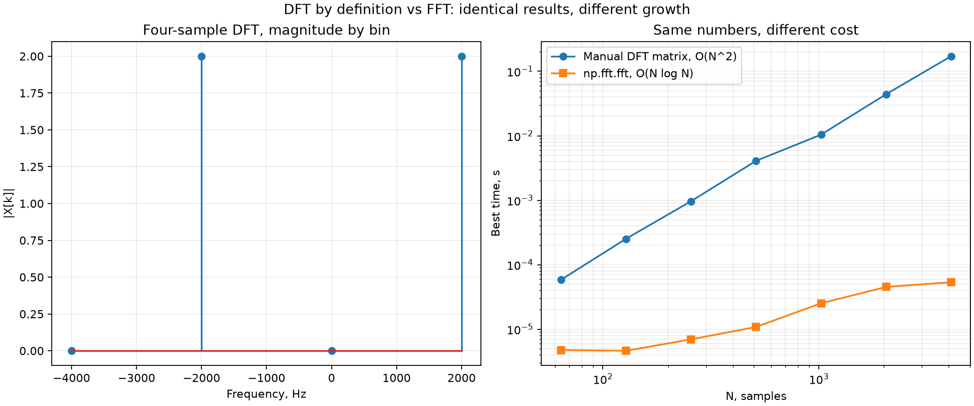
At , the manual method takes several thousand times more time than np.fft.fft, but both return the same numbers within rounding error (). In the rest of the course, we will always calculate the spectrum with np.fft.fft, and use the DFT formula only for explanations and checks on small examples.
Self-check
Take — this is : the same period as in the lesson example, but shifted by a quarter turn. Use the table of reference signals to find .
Only the columns and contribute. ; ; ; . The magnitudes are the same as for the cosine ( at Hz), but the angles are different: and . The quarter-turn shift of the signal shows in the phase of the result.
For the signal from the lesson example (, kS/s), np.fft.fft returns the bins in the order Hz. In which order are the frequencies after np.fft.fftshift, and what is the value of at Hz?
fftshift calculates nothing again — it changes only the order: Hz with the values . The peak of at Hz is still there.
is doubled. By approximately how many times does the time of the DFT from the definition (matrix method) and the time of the FFT increase?
For the DFT from the definition: . For the FFT: — a little more than . For example, from to , the FFT becomes times more expensive. On the lab plot, you see this as the different slopes of the lines.
The butterfly formula uses the same and as the formula for . Why do we not need to calculate a DFT of length again for the second half of the bins?
and are DFTs of length , so and : for the half-length record, the reference signals of bins and differ by an integer number of turns. And the factor differs from the previous one by its sign. Thus one pair , gives two outputs at the same time.