A cosine as a sum of two rotations; complex baseband

The sum of conjugate vectors, and the representation of a signal relative to the tuning frequency.

We add opposite rotations

In the previous lesson, we compared the two directions of rotation. Now we add two conjugate vectors and see how they give a usual real cosine.

For one angle $\theta$ :

z_+=\cos\theta+j\sin\theta,\qquad z_-=\cos\theta-j\sin\theta.

To add complex numbers, we add each coordinate separately:

z_++z_-=(\cos\theta+\cos\theta)+j(\sin\theta-\sin\theta) =2\cos\theta+j0.

The vertical coordinates cancel each other. The horizontal coordinates add, so we get two times the cosine value. To get the cosine itself, we divide the sum by 2:

\boxed{\cos\theta=\frac{e^{j\theta}+e^{-j\theta}}{2}}.

At $\theta=60^\circ$ , this is especially easy to check:

(0.5+j0.866)+(0.5-j0.866)=1+j0.

Half of the sum is $0.5$ , the same as $\cos60^\circ$ .

Angle: 60°

z₊ = 0.500 + j0.866z₋ = 0.500 − j0.866z₊ + z₋ = 1.000 + j0(z₊ + z₋) / 2 = 0.500 + j0

To add vectors geometrically, we move the start of the second vector to the end of the first vector. The dashed copy of $z_-$ on the diagram shows this move. The end of the copy gives the sum $z_++z_-$ ; a darker purple line shows half of the sum.

If you only draw the horizontal projections of the two initial vectors on top of each other, they are the same. To add the coordinates, you need two horizontal steps, one after the other. This is why the sum of the projections in the example is $1$ , although each projection is $0.5$ .

Why each rotation has half of the amplitude

You can divide the sum by 2 at the end, or you can start with two vectors of half length:

A\cos\theta=\frac{A}{2}e^{j\theta}+\frac{A}{2}e^{-j\theta}.

If $\theta$ increases with time, these are two opposite rotations with amplitudes $A/2$ . Their sum always stays on the horizontal axis and oscillates from $-A$ to $+A$ .

This is a mathematical representation of the signal. It will be useful for frequency shift and for spectrum analysis. In the next lesson, we will see that a cosine with amplitude 1 gives two components of 0.5 each in the two-sided spectrum.

We shift the tuning frequency to zero

Let us go back to the receiver tuned to 7.100 MHz. The wanted signal occupies only a few kHz around this frequency. If we shift it to zero, this narrow band sets the processing requirements; after filtering, we can decrease the sample rate.

The reference oscillator LO (local oscillator) sets the tuning frequency. We are interested in the difference:

f_{relative}=f_{RF}-f_{LO}.

Here $f_{RF}$ is the frequency of the input radio signal. For $f_{LO}=7.100$ MHz:

Input frequency	Frequency relative to LO
7.099 MHz	−1 kHz
7.100 MHz	0 Hz
7.101 MHz	+1 kHz

This table gives a frequency plan. It does not mean direct sampling of a MHz signal at a low $F_s$ . In our experiments, we use frequencies that are valid for the selected sample rate.

How a digital mixer works

A digital mixer multiplies the input samples by the samples of a reference signal. To subtract the LO frequency, we select a reference complex rotation with a negative sign:

e^{j2\pi f_{RF}t}\,e^{-j2\pi f_{LO}t} =e^{j2\pi(f_{RF}-f_{LO})t}.

When you multiply, the exponents add. The minus sign of the reference signal is what gives the frequency difference. Multiplication by a positive rotation, on the other hand, would add the LO frequency.

This expression describes the shift of one complex component. A usual real cosine has two components: both move by $-f_{LO}$ , and then a filter selects the necessary band near zero. We will build the full mixer and filter diagram later.

What complex baseband means

Baseband is the band near zero frequency. In our receiver, we get it after the frequency shift and after a filter selects the necessary band. For example, instead of the band around 7.100 MHz, we work with the range from $-3$ to $+3$ kHz.

If both coordinates $I,Q$ represent the signal in this band, we call it complex baseband. We can write a sample as

u[n]=I[n]+jQ[n]=A[n]e^{j\phi[n]}.

Here the letter $u$ only identifies the signal after the frequency shift. The magnitude $A[n]$ shows its current amplitude, and the angle $\phi[n]$ shows its phase relative to the reference oscillator. The amplitude scale depends on the gains selected in the chain.

For one tone with constant amplitude:

Vector behavior after the frequency shift	Meaning
The angle is constant	the tone frequency is equal to the LO frequency
The angle increases at a constant rate	the tone is above the LO
The angle decreases at a constant rate	the tone is below the LO

For a modulated signal, the length and the angle can change in more complex ways: these changes contain the message. One instantaneous angle cannot tell you the frequencies of all the components in a mixture.

Lab: we check the sum of rotations

The script checks the first part of the lesson: the decomposition of the cosine. It does not yet model the shift of a radio signal to zero.

uv run labs/02/03-real-cosine-rotations.py --show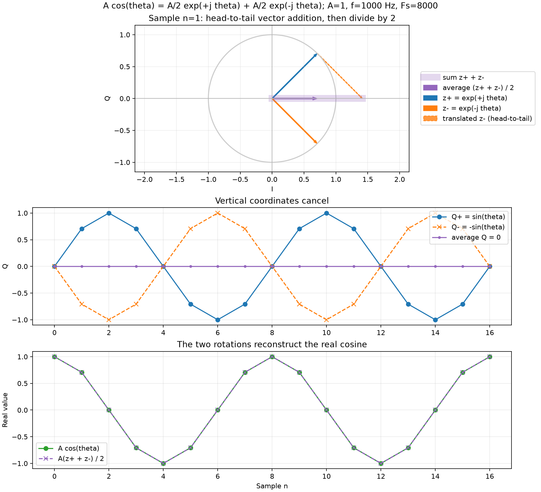

A cosine as a sum of conjugate rotations

Change the amplitude and initial phase:

uv run labs/02/03-real-cosine-rotations.py --amplitude 2 --phase-deg 30 --show --output-dir /tmp/dsp-cosine-pair

The script compares the sum of the two rotations with the initial cosine. The maximum difference must be near zero; a small remainder comes from rounding in the calculations.

Self-check

For $\theta=90^\circ$ , find $z_+=e^{j\theta}$ , $z_-=e^{-j\theta}$ and half of their sum $(z_++z_-)/2$ .

Explanation

$z_+$ points up ( $j$ ), $z_-$ points down ( $-j$ ). Their sum is zero, and this agrees with $\cos90^\circ=0$ : half of the sum of conjugate vectors is always the cosine of the angle.

When you add the conjugate numbers $z$ and $z^*$ , which coordinates cancel and which coordinates add?

Explanation

$z=I+jQ$ , $z^*=I-jQ$ . The sum $2I$ is always a real number. This is why the sum of two opposite rotations stays on the horizontal axis and gives a real cosine.

A cosine has amplitude $4$ . What is the length of each of the two rotating vectors in its decomposition?

Explanation

When both vectors point to the right, their lengths add and give the maximum of the cosine. To get $4$ , each vector must have length $A/2=2$ .

After the shift to zero, the magnitude of one sample became two times larger, and the angle stayed the same. How do $I$ , $Q$ , the magnitude $A$ and the phase $\phi$ change? The initial $I$ and $Q$ are not zero.

Explanation

The vector was stretched two times along the same direction. $A\to2A$ , $\phi$ stays the same, and $I=A\cos\phi$ and $Q=A\sin\phi$ double.

Next lesson: Fourier as a bank of correlators →