The Nyquist frequency: where the phase goes

What is lost exactly at the limit, and why being near it does not mean the signal is lost.

What we saw already

At Fs = 48 kS/s and f = 24 kHz, the point turns by exactly 180° in each interval between measurements. For a cosine with amplitude 1:

Initial phase	First four samples
0°	1, −1, 1, −1
60°	0.5, −0.5, 0.5, −0.5
90°	0, 0, 0, 0

The physical amplitude is the same in all three rows. The difference is where the sampling instants fall. With a phase of 90°, the signal reaches its maximums between the samples, and the ADC sees zero each time.

In NumPy, we give the phase in radians: np.pi / 2 or np.deg2rad(90). The number 90 means 90 radians and gives a very different result. A small remainder near mathematical zero in float64 is computational rounding.

One formula explains all three cases

At the limit f = Fs/2:

x[n]=A\cos(\pi n+\phi).

Expand the cosine of the sum:

x[n]=A\bigl(\cos(\pi n)\cos\phi-\sin(\pi n)\sin\phi\bigr).

For an integer n, always $\sin(\pi n)=0$ , and $\cos(\pi n)=(-1)^n$ . So:

\boxed{x[n]=\underbrace{A\cos\phi}_{C}\,(-1)^n.}

The full record has the form C, −C, C, −C, …. It keeps only one number, C — the product of the amplitude and the cosine of the phase. Without more information, you cannot recover A and φ separately from this record.

This is not a random ADC error: even ideal samples do not contain sufficient information.

Ambiguity also occurs without zeros

Compare two signals at Fs/2:

A = 1, φ = 60° → C = 1 · 0.5 = 0.5;
A = 0.5, φ = 0° → C = 0.5 · 1 = 0.5.

Both give 0.5, −0.5, 0.5, −0.5, …. From the array, you cannot find which amplitude was at the input. And C = 0 can mean that there is no signal, or that there is a non-zero cosine with a phase of 90°.

On the circle, we always see only two opposite points. A longer record does not add new positions.

Lab: compare phases and frequencies

The script plots samples for the phases 0°, 60° and 90° and checks the example with two different amplitudes.

uv run labs/01/03-nyquist.py --show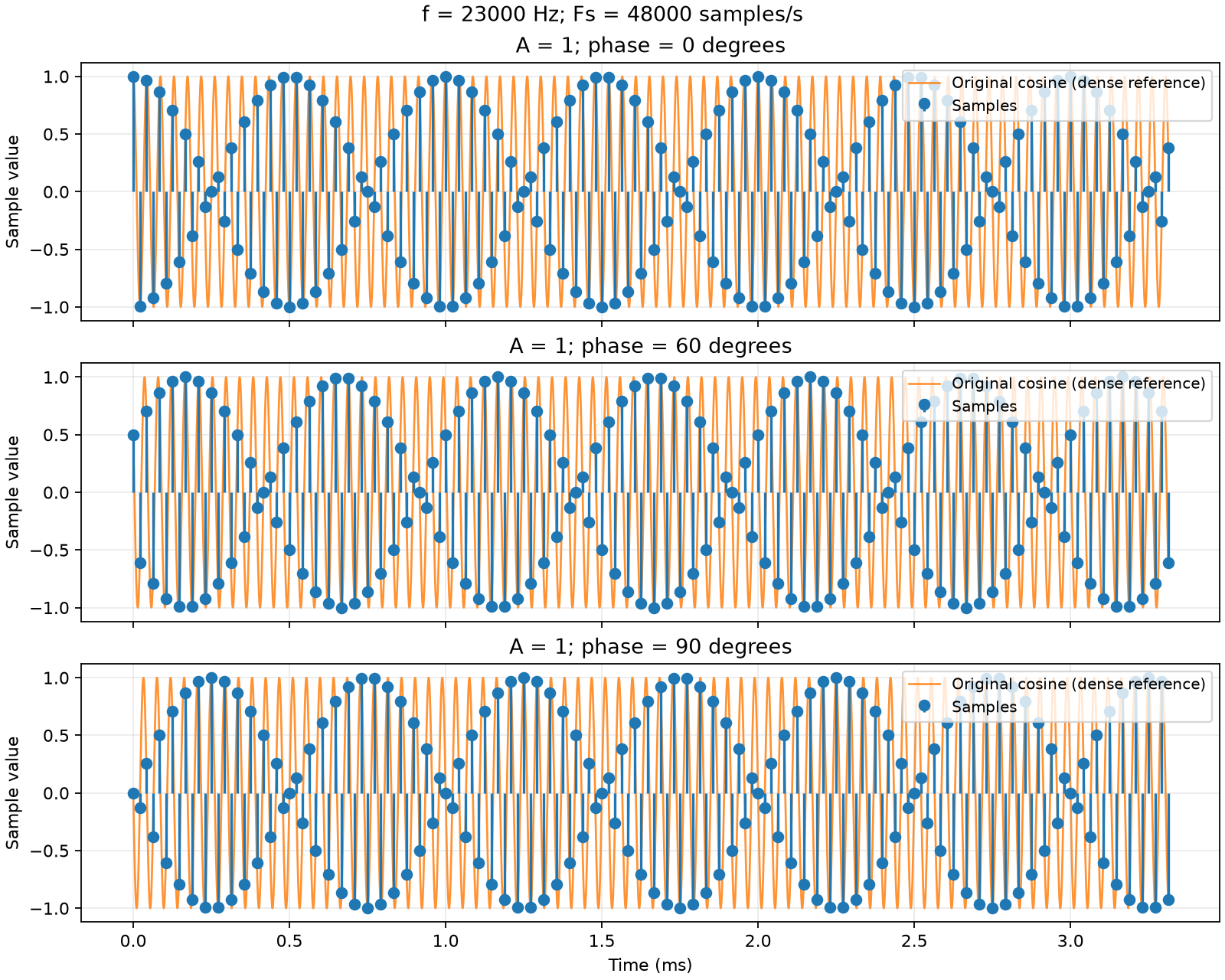

Three phases at the Nyquist frequency

Now decrease the frequency to 23 kHz and keep Fs = 48 kS/s:

uv run labs/01/03-nyquist.py --f 23000 --reference --show --output-dir /tmp/dsp-below-nyquist

The angle step becomes 172.5°, not 180°. The points no longer alternate between only two positions. In particular, with an initial phase of 90°, the samples are no longer all zero. The --reference flag adds the original cosine, calculated on a dense time grid. To look at a few separate periods, add --samples 16.

On a long record, the points can make a pattern that looks like a slowly changing envelope. But the amplitude of the original sinusoid is constant: what changes is the position of the sampling instants relative to its maximums. From the appearance of sparse points, you cannot conclude that reconstruction is impossible.

You can also compare a third case: f = 24 kHz with Fs increased to 96 kS/s.

uv run labs/01/03-nyquist.py --fs 96000 --show --output-dir /tmp/dsp-higher-sample-rate

You get four samples per period and a step of 90°. Even with an initial phase of 90°, we now see 0, −1, 0, +1, …

What the Nyquist condition means

For a real signal with all its frequencies in the band from 0 to $B$ , we use the condition:

F_s > 2B.

Strictly greater protects against our example with a sinusoid exactly at the limit. We assume that the input signal is limited to this band: a high Fs alone does not remove the effect of unknown out-of-band signals.

In the ideal model, a band-limited signal is reconstructed from the complete sequence of samples. This also applies to a 23 kHz sinusoid at $F_s=48$ kS/s: being near the limit does not by itself destroy information. In the lab, the record is finite, and in a device the measurements contain noise — these are additional limits. Straight lines between neighboring points do not give ideal reconstruction.

Why a device has a margin

Before the ADC, you need an analog anti-aliasing filter. A real filter cannot pass everything up to $B$ and immediately suppress everything just above $B$ : between the passband and the stopband there is a transition band. The frequency plan must leave space for the filter roll-off and give sufficient suppression of signals that can alias into the useful band.

This is why “we need a signal up to 20 kHz — so Fs = 40 kS/s” is not correct. Fs = 48 kS/s gives a limit of 24 kHz and some margin, but you must still check that a specific filter is sufficient. There is no single mandatory margin factor for all systems.

Self-check

At Fs = 48 kS/s and f = 24 kHz, we recorded the sequence 0.5, −0.5, 0.5, −0.5, …. The signal is $x[n]=A\cos(\pi n+\phi)$ , which is $x[n]=A\cos\phi\,(-1)^n$ .

From this record, can you say that the amplitude $A$ of the original sinusoid was $0.5$ ?

Explanation

All samples are equal to $\pm C$ , where $C=A\cos\phi$ . One number $C=0.5$ is not sufficient to find two unknowns $A$ and $\phi$ . For example, $A=0.5$ , $\phi=0$ is possible — and an infinite number of other pairs.

Which pair of amplitude and phase, other than $A=0.5$ , $\phi=0$ , also gives the record $0.5,\ -0.5,\ 0.5,\ \ldots$ ?

Explanation

We look for pairs with $A\cos\phi=0.5$ . Possible pairs are $A=1$ and $\phi=\pm60^\circ$ , and also, for example, $A\approx0.71$ and $\phi=\pm45^\circ$ . At the Nyquist frequency, all these signals give the same samples.

We decrease the signal frequency to 23 kHz at the same $F_s=48$ kS/s. What is the angle step between samples $\Delta\theta=360^\circ f/F_s$ now?

Explanation

$\Delta\theta=360^\circ\cdot23/48=172.5^\circ$ . This is $7.5^\circ$ less than half a turn. So after each two samples, the point does not come back exactly to its previous position: it is $15^\circ$ behind.

Do the samples of the 23 kHz signal still follow the sequence $C,-C,C,-C,\ldots$ with a constant $C$ ?

Explanation

The step is $172.5^\circ=180^\circ-7.5^\circ$ . So $x[n]=(-1)^nA\cos(7.5^\circ n-\phi)$ : the sign alternates, and the magnitude changes slowly. In $360^\circ/7.5^\circ=48$ samples, this factor goes through a full cycle. From the samples, you can again find both the amplitude and the phase — being near the limit does not destroy information.

In the next lesson, we separate sampling in time from quantization in amplitude: until now, we used ideal numbers for the sample values.

Next lesson: Quantization: how amplitude becomes a code.