The goal of the first session is to understand what an array of a digital signal contains. We start with one oscillation and learn to calculate its values at selected time instants.
Sinusoid: amplitude, frequency and phase
Imagine a voltage that rises and falls smoothly. The simplest model of this oscillation is:
| Symbol | Meaning | Units |
|---|---|---|
| Time | seconds, s | |
| Peak amplitude | arbitrary units here | |
| Number of full cycles per second | hertz, Hz | |
| Initial phase: the point in the cycle where we start | radians, rad |
One turn is , or radians. In time , the signal makes turns, so the angle changes by . The quantity is the angular frequency; its unit is rad/s.
A cosine is a sinusoidal oscillation. The functions sin and cos differ only by a phase shift. When , the cosine starts at its maximum . When , it starts at zero and first decreases. When , it starts at . The initial phase moves the oscillation in time and keeps its frequency the same.
For example, Hz means 1000 cycles per second. The period of one cycle is:
When , the values change from to . The peak-to-peak range from minimum to maximum is .
From a continuous signal to samples
A computer keeps values only at separate time instants. We measure the signal at equal intervals. This is sampling (time discretization).
The sample rate is the number of measurements per second. One result is a sample. Its index starts at zero:
is the frequency of the oscillation itself, and is the rate of the measurements. When samples per second, the interval is μs. For a kHz sinusoid, one period contains sample periods. This ratio does not have to be an integer.
How to calculate a specific sample
For each index , do the same steps:
- Find the sampling instant: .
- Find the angle: .
- Calculate the value: .
For example, with , , , , sample is at s. The angle is , or , and the value is approximately .
In NumPy, you give the angle in radians:
import numpy as np
import matplotlib.pyplot as plt

fs = 48_000
f = 1_000
n = np.arange(96)          # indices 0 ... 95
t = n / fs                # sampling instants, seconds
x = np.cos(2 * np.pi * f * t)

plt.stem(t * 1000, x)
plt.xlabel('Time (ms)')
plt.ylabel('Amplitude')
plt.show()
The first values are: [1, 0.991445, 0.965926, 0.923880, ...]. For now, we model ideal measurements. We discuss the limit of amplitude precision in the lesson on quantization.
A record of samples at kS/s lasts ms. The last sample is at ms; the moment ms already belongs to the next block. This is why we make the time axis as np.arange(N) / fs.
A circle as a model of oscillation
A point on a circle of radius 1 has the horizontal coordinate . On the right, this coordinate is ; at the top, ; on the left, ; at the bottom, . When the point turns at a constant speed, the horizontal coordinate changes as a cosine.
This circle helps you imagine how the voltage changes. The frequency sets the number of turns per second. During sampling, we record the horizontal coordinate times per second. In the time between two measurements, the point moves through the angle
Take kHz and kS/s. The angle step is . The first six samples are: . The next sample is again.
The slider selects the sample index. The green dot shows the position on the circle. The orange square shows its horizontal coordinate, which is the value we record.
Lab: change the sinusoid parameters
From the project directory, run the script:
uv run labs/01/01-sine-sampling.py --showThe dependencies are declared inside the script; uv prepares the environment. At the start of the file are the parameters FS, FREQUENCY, AMPLITUDE, PHASE, N. Change them one at a time:
- Run with the initial values Hz, , , .
- Set
FREQUENCY = 2_000: how many cycles fit into 2 ms now? - Set 1000 Hz again and set
AMPLITUDE = 0.5: how do the maximum and minimum change? - Set
PHASE = np.pi / 2: what is the first sample? A small remainder near instead of zero comes from rounding during the calculation.
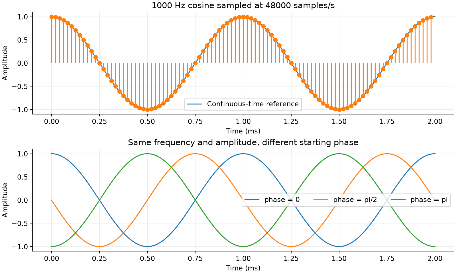
On the top plot, the smooth line is calculated on a dense time grid, and the dots are our 96 samples. The bottom plot compares three fixed initial phases.
For a separate experiment with the circle:
uv run labs/01/circle-sampling.py --showFor a step-by-step calculation of specific samples:
uv run labs/01/sample-value.py --fs 8000 --f 1000 --n 0 1 2 3Can different signals give the same array?
The second figure of the main lab compares cosines at 20 and 28 kHz with kS/s. Both have amplitude 1 and initial phase 0.
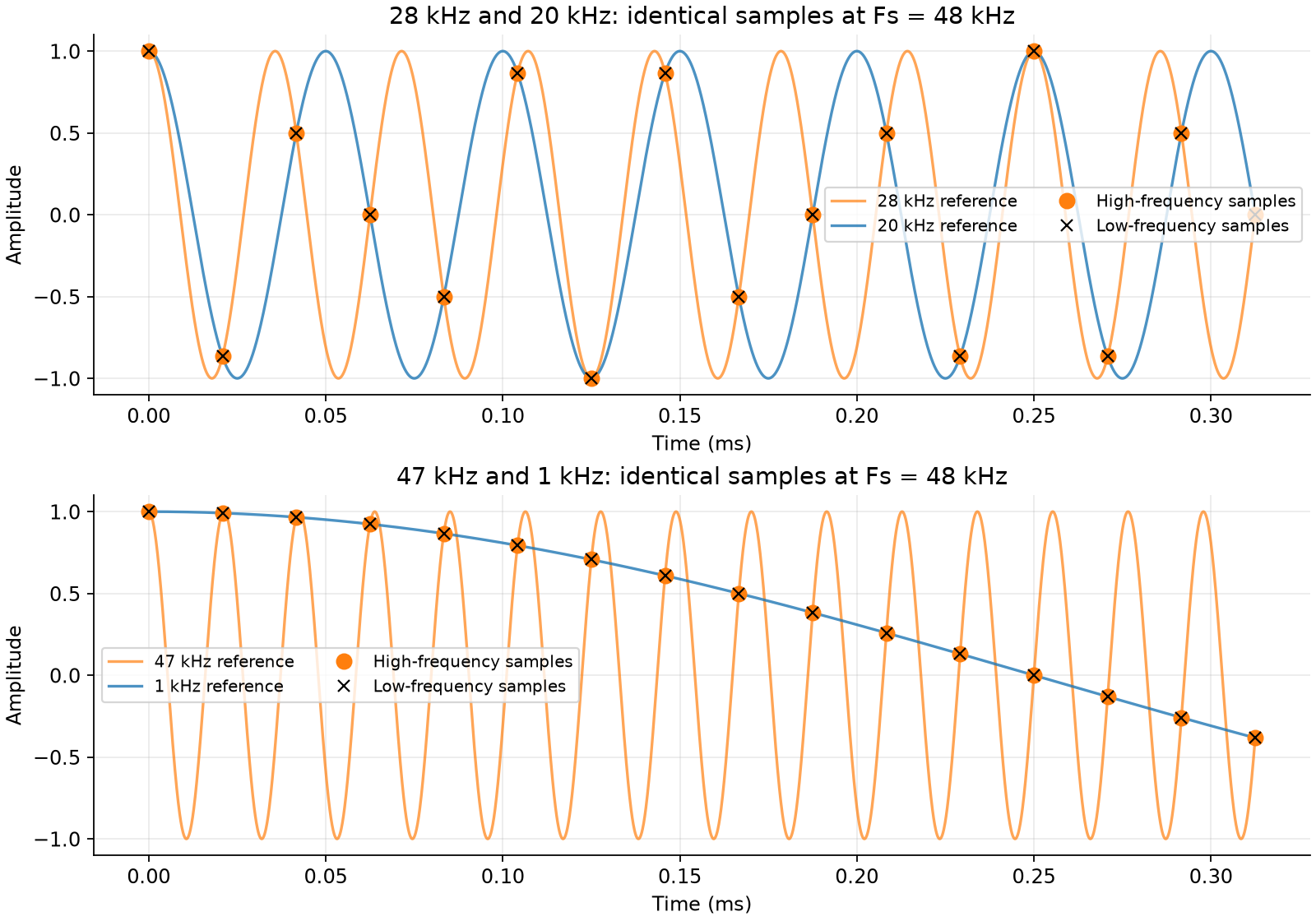
The curves are different, but their values at the sampling instants are the same. The same thing occurs with the pair 1 and 47 kHz. This is aliasing: from the samples, you cannot find the original frequency without ambiguity. In the next lesson, we find the cause with the circle and check it with calculations.
For this experiment, keep FS = 48_000: the frequency pairs in the script are selected for this sample rate.
Self-check
Given: kHz, kS/s, , . The signal is .
What is the period of the sinusoid in microseconds?
The period is the time of one full turn: s µs. The sample rate has no effect on the period — it sets only how often we measure the signal.
How many sample periods fit into one period of the signal?
µs, and µs. The ratio is . In one interval, the point turns by .
What is the first sample ?
When , the angle is equal to the initial phase: . The point on the circle is on the right, and its horizontal coordinate is . Multiply by the amplitude: .
We change only the initial phase . What happens to the period and the interval between samples ?
The phase sets the angle where the rotation starts. The sample values change, for example , but the speed of rotation and the sampling instants do not change.
First answer without Python, then check the calculation in the lab. The sinusoid generator will be useful to test the next blocks of the transceiver.