← A cosine as a sum of two rotations; complex baseband
Why we need a spectrum
Imagine that two signals come into the receiver at the same time. Each sample contains their sum. On a time plot, we see the shape of the total oscillation, but it can be difficult to find the frequencies of the separate components from it.
The spectrum helps to answer two questions: which frequencies are in the signal, and what are the amplitudes of its components?
In the previous lesson, we shifted the frequency of a signal by multiplication with a complex rotation. Now we use the same operation for measurement: we try to cancel the rotation of a selected frequency and see what we get when we add the samples.
A complex sample on the I/Q plane
We start with one complex tone — a signal whose phasor rotates at a constant rate and keeps its length. Each sample of it is a complex number:
On the diagram, this is a vector from the origin to the point . Its length shows the magnitude of the number, and its angle from the positive axis shows the phase. When we change the index , we look at consecutive samples of one signal.
For our example, we set:
- signal frequency kHz;
- sample rate kS/s;
- amplitude and initial phase ;
- eight samples, from to .
In the interval between samples, the vector turns counterclockwise by
The first samples are:
| Value | Vector direction | |
|---|---|---|
| 0 | right | |
| 1 | up | |
| 2 | left | |
| 3 | down | |
| 4 | right again |
How to test one frequency
We want to find out if the input signal has a component at the frequency kHz. For this, the program makes a reference signal: a complex exponential. Its amplitude is , its initial phase is , and it rotates clockwise: by per sample.
Here it is important to keep apart the analysis frequency kHz and the frequency of the reference rotation itself, kHz. We need the opposite sign to cancel the rotation of the input signal.
We multiply the samples that have the same index:
where is a sample of the reference signal and is the result. This is the same operation that we called a digital mixer. When you multiply complex numbers, their magnitudes multiply and their angles add.
| Input | Reference signal | Product | |
|---|---|---|---|
| 0 | |||
| 1 | |||
| 2 | |||
| 3 |
For example, at the angles add like this: . The result is the number , and its vector points to the right.
All eight output samples are equal to . Thus their sum is . Geometrically, we add eight unit vectors: we move the start of each next vector to the end of the previous one. The result is a vector of length .
A correlator does exactly these two actions: it multiplies the input samples by the reference samples, then adds the results.
What we get at a different analysis frequency
Now we test kHz. The reference rotation is per sample, and the input rotation is . After the multiplication, a rotation of remains, which is the frequency kHz.
The eight output samples have these angles:
n:      0    1    2     3     4     5     6     7
angle:  0°  45°  90°  135°  180°  225°  270°  315°
These vectors point in directions spread evenly around the circle. Each vector has an opposite one: for example, and . When we add them, they cancel each other. If you put them one after another, you get a closed octagon, and the sum is zero.
In this example, the sum is exactly zero because of the frequencies and the number of samples that we selected. An arbitrary frequency that does not match does not have to give a zero sum. If the cancellation is not complete, part of the result remains; later we will study this as spectral leakage.
Input signal: +2 kHz, Fs = 8 kS/s. Amplitude 1, initial phase 0°.
Start with the analysis frequency kHz and change the sample index. The top row shows the input vector, the reference vector and the result of their multiplication. The input and the reference change direction, but the result is each time.
Then select kHz. Now the direction of the result vector also changes. The bottom left shows all eight results from a common origin; the bottom right shows their consecutive addition. When the frequencies match, the eight vectors on the left lie on top of each other, so you see only one.
The same operation in formulas
For a complex tone with frequency , amplitude and initial phase :
To test the frequency , we make a reference signal:
When we multiply, the angles add, so the difference of the frequencies remains:
At , each result is the same number . Its vector points to the right only when the initial phase is zero, as in our example. With a different phase, all output vectors point at a different common angle. In both cases, the length of the sum is , where is the number of samples.
The output of one correlator
In the general case, we write the input sequence as : it can be one tone or a sum of several tones, a real or a complex signal. One formula gives the multiplication and the addition:
The symbol means “add the results for all from to ”. The output is one complex number .
For a single complex tone at the analysis frequency:
- the magnitude is , so division by gives the amplitude ;
- the angle of this number is the initial phase of the tone.
For a mix of signals, the correlator adds the contributions of all components. In our examples, we selected the frequencies so that the components that do not match give a zero contribution. With other frequencies and record lengths, the measurement can be less accurate.
From one correlator to the DFT
To make a spectrum, we repeat the measurement for a set of frequencies. The DFT — the discrete Fourier transform — uses analysis frequencies with the step
For example, for eight samples at kS/s, the step is kHz. When we put the negative frequencies on the left, the set is:
−4, −3, −2, −1, 0, +1, +2, +3 kHzHere we wrote the Nyquist frequency as kHz. We do not add the value kHz separately: on the sample grid, these two rotations are the same.
You can write each analysis frequency as . When we put it into the previous formula, we get:
In this example, goes from to . Indices that differ by give the same reference samples: the added angle is an integer number of turns, . Thus you can also number the results from to , as NumPy does. The output is eight complex numbers, one for each analysis frequency. Their magnitudes give the magnitude spectrum.
The FFT is a fast algorithm that calculates the same DFT. The function np.fft.fft() returns the frequencies in a different order: first zero and the positive frequencies, then the negative ones. In the lab, np.fft.fftshift() changes the order of the results for a plot with the negative frequencies on the left. In the next lesson, we will study the indices and calculate a short DFT in detail.
Why a cosine with amplitude 1 gives two peaks of 0.5
In the previous lesson, we wrote a real cosine as a sum of two rotations in opposite directions:
The correlator at picks up one of these rotations, and the correlator at picks up the other. The amplitude of each is .
The lab plot shows : the magnitude of the DFT result divided by the number of samples. Thus, for frequencies that are exactly on the DFT grid, we get:
| Original cosine | Peak at the positive frequency | Peak at the negative frequency |
|---|---|---|
| kHz, amplitude | at kHz | at kHz |
| kHz, amplitude | at kHz | at kHz |
This is a two-sided magnitude spectrum. Its peaks show the amplitudes of the complex rotations that add up to the original cosines.
You can also make a single-sided magnitude spectrum of a real signal: keep the positive frequencies and double their values. Then in our example we see and . We do not double zero frequency and the Nyquist frequency, because they do not have a separate paired component. In this lesson, we keep both sides to keep the link with the two directions of rotation.
Python lab
The script combines two experiments. Run it from the project directory:
uv run labs/03/01-frequency-probe.py --showThe top row tests one complex tone. Here the parameters are different from the interactive diagram: input frequency kHz, number of samples , sample rate kS/s.
- The left plot shows and of the input samples in time.
- The center plot shows the consecutive addition of the results for the analysis frequency kHz. All 32 results are equal to , and the sum is .
- The right plot shows the same addition for the analysis frequency kHz. The remaining frequency is kHz. The sum is near zero; the small error comes from floating-point calculation.
The bottom row analyzes the sum of two real cosines:
On the plot Two real cosines and their sum, dashed lines show the original cosines. The black line is their sum, calculated on a dense time grid to draw a continuous curve. The blue dots are 32 samples of this sum at kS/s. These are the values that go into the DFT.
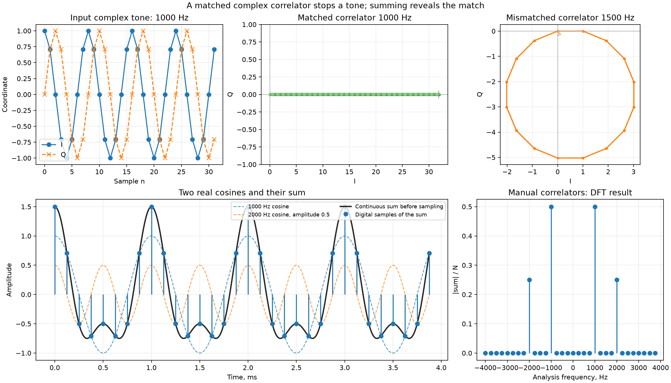
The bottom right plot is the two-sided spectrum of the sum. The step of the analysis frequencies is Hz. Both original frequencies are exactly on this grid. Thus you see four peaks: at kHz with height and at kHz with height .
The program calculates the DFT directly: for each frequency, it multiplies the samples by the reference signal and adds them. Then it compares the result with np.fft.fft().
Self-check
For questions 1–3, we use a complex tone of kHz with amplitude and initial phase . The sample rate is kS/s. We take eight samples, . The reference signal has amplitude , initial phase , and a frequency opposite to the analysis frequency. We write the result of the multiplication as .
We test the frequency kHz. Which frequency remains in after the multiplication?
The input turns by per sample, and the reference turns by . When we multiply, the angles add, and per sample remains. This is the frequency Hz.
For the same test, find and the sum of all eight output samples.
, , , . All eight vectors point to the right, and their sum is .
Now we test kHz. By how many degrees and in which direction does turn per sample, and why is the sum of eight samples equal to zero?
The remaining frequency kHz is a rotation of per sample. The eight vectors at the angles make pairs of opposite directions. When you put them one after another, they close an octagon, and the sum is zero.
We replace the input with a real cosine of kHz with amplitude . Where do the peaks of the two-sided spectrum appear, and what is their height, if the vertical axis shows ?
The cosine breaks down into rotations at kHz and kHz with amplitudes . The correlator at each of these frequencies picks up one rotation: .